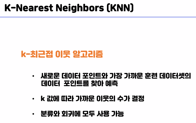
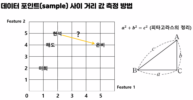
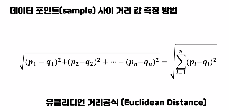
KNN 모델
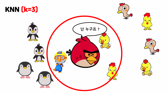
펭귄은 왼쪽에 분포 / 닭은 오른쪽에 분포
k = 3일때 -> 가장 가까운 것들 3개를 골라서 과반수인 닭으로 인식한다
수가 같다면 더 가까운것으로 인식
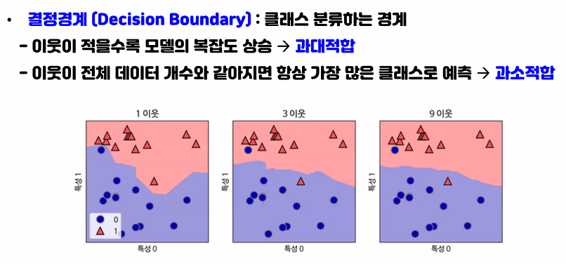
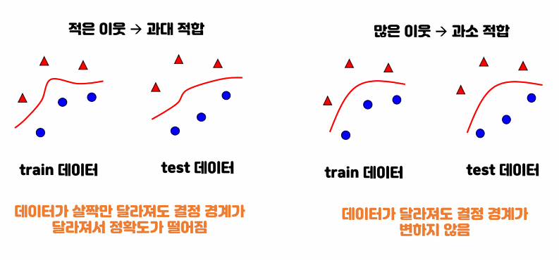
이웃이 적을수록 == k값이 적을수록 (같은말)
그림에서 k=3 / 이웃이 3일때 결정경계가 좀 더 느슨해졌다.
왼쪽은 1차원 / 차원이 늘어갈 수 록 오른쪽 식으로


BMI 실습
import pandas as pd
from sklearn.neighbors import KNeighborsClassifier
data = pd.read_csv('./data/bmi_500.csv',index_col='Label')
data.head()
Gender	Height	Weight
Label
Obesity	Male	174	96
Normal	Male	189	87
Obesity	Female	185	110
Overweight	Female	195	104
Overweight	Male	149	61
data.info()
<class 'pandas.core.frame.DataFrame'>
RangeIndex: 500 entries, 0 to 499
Data columns (total 4 columns):
 #   Column  Non-Null Count  Dtype
---  ------  --------------  -----
 0   Gender  500 non-null    object
 1   Height  500 non-null    int64
 2   Weight  500 non-null    int64
 3   Label   500 non-null    object
dtypes: int64(2), object(2)
memory usage: 15.8+ KB
data.index.unique()
Index(['Obesity', 'Normal', 'Overweight', 'Extreme Obesity', 'Weak',
       'Extremely Weak'],
      dtype='object', name='Label')
각 비만도 등급별 시각화
import matplotlib.pyplot as plt
data.loc['Obesity']
	Gender	Height	Weight
Label
Obesity	Male	174	96
Obesity	Female	185	110
Obesity	Female	169	103
Obesity	Female	159	80
Obesity	Female	169	97
...	...	...	...
Obesity	Male	146	85
Obesity	Female	188	115
Obesity	Male	173	111
Obesity	Male	198	136
Obesity	Female	184	121
130 rows × 3 columns
def myScatter(label, color):
l = data.loc[label]
plt.scatter(l['Weight'],l['Height']
, c = color, label=label) # plt.scatter(x축, y축, c= 컬러설정, label = 라벨적는곳)
plt.figure(figsize=(5,5))
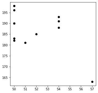
myScatter('Extremely Weak','black')
plt.show()
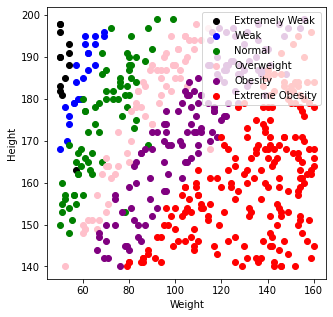
plt.figure(figsize=(5,5))
myScatter('Extremely Weak','black')
myScatter('Weak','blue')
myScatter('Normal','green')
myScatter('Overweight','pink')
myScatter('Obesity','purple')
myScatter('Extreme Obesity','red')
plt.legend(loc='upper right')
plt.xlabel('Weight')
plt.ylabel('Height')
plt.show()
문제와 답으로 분리해보기 ( 답: Label, 문제: 키, 몸무게)
data1 = pd.read_csv('./data/bmi_500.csv')
data1.head()
Gender	Height	Weight	Label
0	Male	174	96	Obesity
1	Male	189	87	Normal
2	Female	185	110	Obesity
3	Female	195	104	Overweight
4	Male	149	61	Overweight
X = data1.iloc[:,1:3]
y = data1.iloc[:,3]
print(X.shape)
print(y.shape)
(500, 2)
(500,)
train, test 분리 : 훈련셋과 평가셋으로 분리
- 7:3 or 7.5:2.5
X_train = X.iloc[:350, :] #훈련셋 행 350개 -> 전체의 70%
X_test = X.iloc[350:, :]
y_train = y[:350]
y_test = y[350:]
print(X_train.shape)
print(X_test.shape)
print(y_train.shape)
print(y_test.shape)
(350, 2)
(150, 2)
(350,)
(150,)
모델설정
k_model = KNeighborsClassifier(n_neighbors=10) # 이 k=10 의 값에 따라 정확도가 달라진다
학습, 예측
평가
k_model.fit(X_train,y_train) # 학습할 데이터는 문자형데이터, 결측치가 있으면 안된다.KNeighborsClassifier(n_neighbors=10)
pre = k_model.predict(X_test) # 테스트 문제 넣고
from sklearn import metrics
metrics.accuracy_score(pre,y_test) # 평가시 순서는 상관없다.
0.9333333333333333활용
k_model.predict([[179,84]])
array(['Overweight'], dtype=object)map()활용해 남자 -> 0 여자->1로 변경
X = data.iloc[:,:3]
y = data.index

dic = {
    'Male':0,
    'Female':1
}

X['Gender'] = X['Gender'].map(dic)

X
Gender Height Weight
Label
Obesity 0 174 96
Normal 0 189 87
Obesity 1 185 110
Overweight 1 195 104
Overweight 0 149 61
... ... ... ...
Extreme Obesity 1 150 153
Obesity 1 184 121
Extreme Obesity 1 141 136
Extreme Obesity 0 150 95
Extreme Obesity 0 173 131
500 rows × 3 columnsIris 데이터 실습
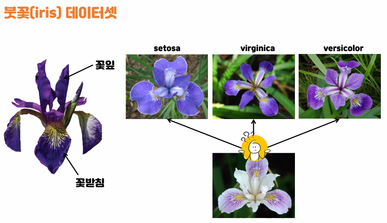
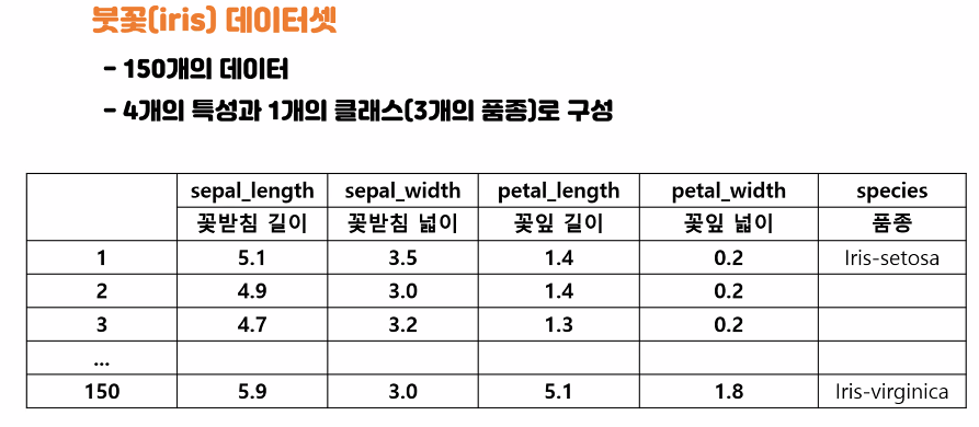
목표
- 봇꽃의 꽃잎 길이, 꽃잎 너비, 꽃받침 길이, 꽃받침 너비 특징을 활용해 3가지 품종을 분류해보자
from sklearn.datasets import load_iris
import pandas as pd
import matplotlib.pyplot as plt
from sklearn.neighbors import KNeighborsClassifier
from sklearn import metrics
i_data = load_iris()
i_data
i_data.keys()
dict_keys(['data', 'target', 'frame', 'target_names', 'DESCR', 'feature_names', 'filename'])i_data['data'] #i_data.data(키값)
array([[5.1, 3.5, 1.4, 0.2],
       [4.9, 3. , 1.4, 0.2],
       [4.7, 3.2, 1.3, 0.2],
       [4.6, 3.1, 1.5, 0.2],
       [5. , 3.6, 1.4, 0.2],
       [5.4, 3.9, 1.7, 0.4],
       ....................
i_data['feature_names']
['sepal length (cm)',
 'sepal width (cm)',
 'petal length (cm)',
 'petal width (cm)']
print(i_data.DESCR) # 전체 구조 출력
.. _iris_dataset:

Iris plants dataset
--------------------

**Data Set Characteristics:**

    :Number of Instances: 150 (50 in each of three classes)
    :Number of Attributes: 4 numeric, predictive attributes and the class
    :Attribute Information:
        - sepal length in cm
        - sepal width in cm
        - petal length in cm
        - petal width in cm
        - class:
                - Iris-Setosa
                - Iris-Versicolour
              .....................
데이터 셋 구성하기
- 문제와 답 분리
X = i_data['data'] # i_data.data
y = i_data['target'] # i_data.target
- train, test 분리
X_train = X[:105]
X_test = X[105:]
y_train = y[:105]
y_test= y[105:]   # 이렇게 슬라이싱하면 0,1이 많고 2가 없어서 다양성이 떨어진다


from sklearn.model_selection import train_test_split  # 순서를 랜덤으로 섞어주는 라이브러리


X_train, X_test, y_train, y_test = train_test_split(X,y, test_size=0.3, random_state = 1)
     #X_train, test 순서들 꼭 지키기
     # test_size 로 훈련셋70 테스트셋 30 설정 / random_state = 숫자로 고정되어 랜덤화

print(X_train.shape)
print(X_test.shape)
print(y_train.shape)
print(y_test.shape)
(105, 4)
(45, 4)
(105,)
(45,)y_test
array([0, 1, 1, 0, 2, 1, 2, 0, 0, 2, 1, 0, 2, 1, 1, 0, 1, 1, 0, 0, 1, 1,
       1, 0, 2, 1, 0, 0, 1, 2, 1, 2, 1, 2, 2, 0, 1, 0, 1, 2, 2, 0, 2, 2,
       1])
모델링
- knn 모델 만들기 k값 3
- 학습
- 예측
- 평가
k_model = KNeighborsClassifier(n_neighbors=3)

k_model.fit(X_train, y_train)
  KNeighborsClassifier(n_neighbors=3)

pre = k_model.predict(X_test)
metrics.accuracy_score(y_test,pre)0.9777777777777777k_model.score(X_test,y_test) # predict과정 없이 테스트 문제, 답만 넣고 평가 가능하다
0.9777777777777777최적의 k값 찾기
test_l = []
train_l = []

for k in range(1,80,2):
    m = KNeighborsClassifier(n_neighbors= k)
    m.fit(X_train, y_train)

    train_pre = m.predict(X_train)
    test_pre = m.predict(X_test)

    s1 = metrics.accuracy_score(train_pre, y_train)
    s2 = metrics.accuracy_score(test_pre, y_test)

    train_l.append(s1)
    test_l.append(s2)
plt.figure(figsize=(10,10))
plt.plot(range(1,80,2),train_l, label='train')
plt.plot(range(1,80,2),test_l, label='test')
plt.legend()
plt.show()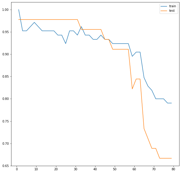
k=1일때 -> train보다 test 성능이 떨어지는 과대적합
2~30은 일반화 구간 후
k=30정도 이후 부터 과소적합구간
-> * 회귀일때는 과반수가 아니라 평균값으로 계산한다
'빅데이터 서비스 교육 > 머신러닝' 카테고리의 다른 글
| Cross validation (0) | 2022.06.24 |
|---|---|
| 머신러닝 Decision Tree (0) | 2022.06.24 |
| Decision Tree (0) | 2022.06.23 |
| 머신러닝 데이터 예측 (KNN모델) (0) | 2022.06.23 |
| 머신러닝 (0) | 2022.06.21 |