예제 타이타닉 생존자 예측분석

빅데이터 서비스 교육/머신러닝

예제 타이타닉 생존자 예측분석

Manly 2022. 6. 24. 12:52

타이타닉 생존자 예측분석

1. 목표

타이타닉 데이터를 학습해서 생존자/사망자를 예측해보자
머신러닝의 전체 과정을 진행해보자.

2. 데이터 수집

import numpy as np
import pandas as pd
import matplotlib.pyplot as plt
import seaborn as sns # 시각화 라이브러리
from sklearn.tree import export_graphviz

import pandas as pd
train = pd.read_csv('./data/titanic/train.csv', index_col = 'PassengerId')
test = pd.read_csv('./data/titanic/test.csv', index_col = 'PassengerId')

3. 데이터 전처리

결측치 채우기

train.info() # Age, Cabin, Embarked의 결측치들을 채워야 한다.

<class 'pandas.core.frame.DataFrame'>
Int64Index: 891 entries, 1 to 891
Data columns (total 11 columns):
 #   Column    Non-Null Count  Dtype  
---  ------    --------------  -----  
 0   Survived  891 non-null    int64  
 1   Pclass    891 non-null    int64  
 2   Name      891 non-null    object 
 3   Sex       891 non-null    object 
 4   Age       714 non-null    float64
 5   SibSp     891 non-null    int64  
 6   Parch     891 non-null    int64  
 7   Ticket    891 non-null    object 
 8   Fare      891 non-null    float64
 9   Cabin     204 non-null    object 
 10  Embarked  889 non-null    object 
dtypes: float64(2), int64(4), object(5)
memory usage: 83.5+ KB

Age 결측치 채우기

다른 컬럼간의 상관관계를 이용해 결측치를 채워보자

train.corr()         # corr() -> 상관관계를 볼 수 있다 (수치데이터만 볼 수 있다)
                     # -1 ~ 1  -> 1로 갈수록 강한 상관관계 -> 양으로   / 0이면 상관이 없다
                     # -1도 강한 상관관계    -> 음으로 (ex 원수여도 관계는 있다 나쁜쪽으로)
                     # 0.3 ~ 0.5 약한 상관관계  / 0.7이상 강한 상관관계

Survived	Pclass	Age	SibSp	Parch	Fare
Survived	1.000000	-0.338481	-0.077221	-0.035322	0.081629	0.257307
Pclass	-0.338481	1.000000	-0.369226	0.083081	0.018443	-0.549500
Age	-0.077221	-0.369226	1.000000	-0.308247	-0.189119	0.096067
SibSp	-0.035322	0.083081	-0.308247	1.000000	0.414838	0.159651
Parch	0.081629	0.018443	-0.189119	0.414838	1.000000	0.216225
Fare	0.257307	-0.549500	0.096067	0.159651	0.216225	1.000000

Pclass가 Age와 가장 높은 상관관계를 갖는다.
성별을 함께 활용해보자

# pivot table 활용

pt1 = train.pivot_table(values = 'Age', index = ['Pclass','Sex'], aggfunc='mean')
pt1

Age
Pclass	Sex	
1	female	34.611765
male	41.281386
2	female	28.722973
male	30.740707
3	female	21.750000
male	26.507589

pt1.loc[1,'female'] # 인덱스가 2개이기때문에 2개값 필요

Age    34.611765
Name: (1, female), dtype: float64

def fill_age(row):
    # 만약 나이가 결측치라면 피봇테이블에서 값을 가져온다.
    if np.isnan(row['Age']):          #np.isnan() -> 값이 없나?
        return pt1.loc[row['Pclass'],row['Sex']]
    else:
        return row['Age']

train['Age'] = train.apply(fill_age, axis = 1).astype('float64')

train.info()

<class 'pandas.core.frame.DataFrame'>
Int64Index: 891 entries, 1 to 891
Data columns (total 11 columns):
 #   Column    Non-Null Count  Dtype  
---  ------    --------------  -----  
 0   Survived  891 non-null    int64  
 1   Pclass    891 non-null    int64  
 2   Name      891 non-null    object 
 3   Sex       891 non-null    object 
 4   Age       891 non-null    float64
 5   SibSp     891 non-null    int64  
 6   Parch     891 non-null    int64  
 7   Ticket    891 non-null    object 
 8   Fare      891 non-null    float64
 9   Cabin     204 non-null    object 
 10  Embarked  889 non-null    object 
dtypes: float64(2), int64(4), object(5)
memory usage: 83.5+ KB

train의 Age 결측치를 채웠다

Embarked 채우기

train['Embarked'].value_counts()
S    644
C    168
Q     77
Name: Embarked, dtype: int64

test['Embarked'].value_counts()
S    270
C    102
Q     46
Name: Embarked, dtype: int64


# Embarked 컬럼은 결측치가 2개 -> 가장 많은 S로 그냥 채워준다
train['Embarked'] = train['Embarked'].fillna('S')   
# .fillna('채울값') -> 결측치가 채울값으로 채워진다

Fare 채우기

test.info()  # train에는 Fare 결측치 없다

# Pclass와 Sex 컬럼 이용하여 피봇테이블 만들기
pt2 = test.pivot_table(values='Fare', index=['Pclass','Sex'], aggfunc='mean')
pt2

Fare
Pclass	Sex	
1	female	115.591168
male	75.586551
2	female	26.438750
male	20.184654
3	female	13.735129
male	11.826350

test[test['Fare'].isnull()]

Pclass	Name	Sex	Age	SibSp	Parch	Ticket	Fare	Cabin	Embarked
PassengerId										
1044	3	Storey, Mr. Thomas	male	60.5	0	0	3701	NaN	NaN	S

test['Fare'] = test['Fare'].fillna(12.661633)

Cabin 채우기¶

train['Cabin'].value_counts()

B96 B98        4
G6             4
C23 C25 C27    4
C22 C26        3
F33            3
              ..
E34            1
C7             1
C54            1
E36            1
C148           1
Name: Cabin, Length: 147, dtype: int64

train['Deck'] = train['Cabin'].str[0] # C85, C7등으로 있는걸 C만 인덱싱하기위해 train['Cabin']를 str[0]으로 인덱싱
test['Deck'] = test['Cabin'].str[0]

train['Deck'].value_counts()

C    59
B    47
D    33
E    32
A    15
F    13
G     4
T     1
Name: Deck, dtype: int64

train['Deck'] = train['Deck'].fillna('M') # 가데이터 'M'으로 일단 결측치를 채워서 사용
test['Deck'] = test['Deck'].fillna('M')

train.drop('Cabin', inplace = True, axis=1) # 바로 삭제 적용 -> inplace = True
test.drop('Cabin', inplace = True, axis=1)

데이터 탐색

Deck 시각화

sns.countplot(data = train, x='Deck', hue = 'Survived')
# seaborn라이브러리를 이용한 시각화
# 범주형 데이터일 때 countplot을 쓴다

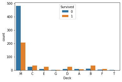
Deck컬럼의 M값에서 사람이 많이 사망했다.
C, E, D, B, F에서 상대적으로 생존한 사람이 더 많다.

Pclass 시각화

# x축 pclass hue survived
sns.countplot(data = train, x='Pclass', hue='Survived')

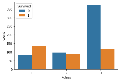
3등석 사람들이 많이 죽었다.

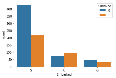
Sex, Embarked 시각화 해보기

sns.countplot(data=train,x='Sex', hue='Survived')

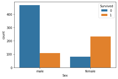
sns.countplot(data=train, x='Embarked', hue='Survived')

Age 시각화

# 수치형 데이터는 violinplot()을 이용
plt.figure(figsize=(15,5))
sns.violinplot(data =train,
              x= 'Sex',
              y= 'Age',
              hue= 'Survived',
              split=True)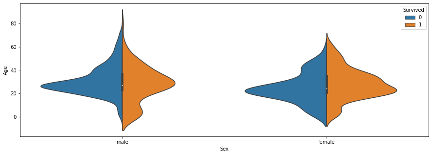

어린아이 중에서는 여자아이가 더 많이 사망했다. (시대적 배경 영향)
20~40대 사이는 두 성별모두 많이 사망

Fare 시각화

plt.figure(figsize=(15,5))
sns.violinplot(data =train,
              x= 'Sex',
              y= 'Fare',
              hue= 'Survived',
              split=True)

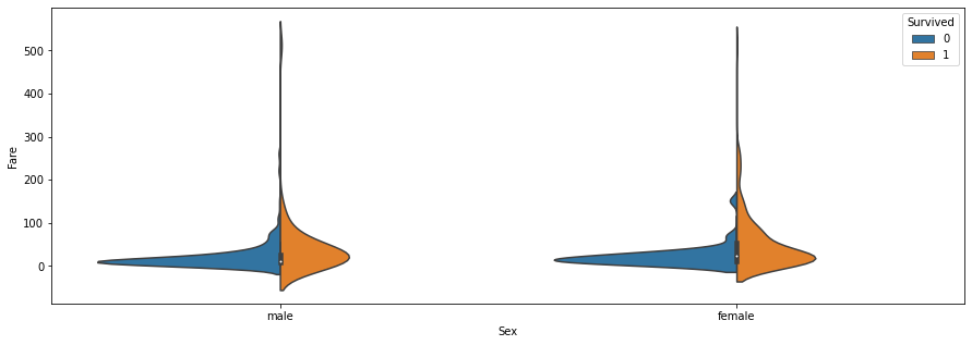
요금이 싼사람은 많이 죽었다.

Parch, SibSp - 부모자식, 형제자매 배우자수¶

특성공학 : Parch, SibSp 두 컬럼을 더하면 -> 가족의 인원수라는 새로운 컬럼 생성
+1로 자기자신 추가

train['Family'] = train['Parch'] + train['SibSp'] + 1
test['Family'] = test['Parch'] + test['SibSp'] + 1

sns.countplot(data=train, x='Family', hue='Survived')

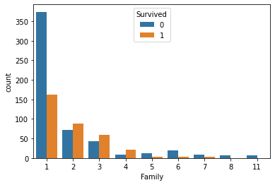
1명일때는 죽은 비율이 높다, 2~4명일때는 산 비율이 높다. 5명이상일때는 사망비율이 높다.

Name 시각화

train['Name']

PassengerId
1                                Braund, Mr. Owen Harris
2      Cumings, Mrs. John Bradley (Florence Briggs Th...
3                                 Heikkinen, Miss. Laina
4           Futrelle, Mrs. Jacques Heath (Lily May Peel)
5                               Allen, Mr. William Henry
                             ...                        
887                                Montvila, Rev. Juozas
888                         Graham, Miss. Margaret Edith
889             Johnston, Miss. Catherine Helen "Carrie"
890                                Behr, Mr. Karl Howell
891                                  Dooley, Mr. Patrick
Name: Name, Length: 891, dtype: object

train['Name'].iloc[1].split(',')[1].split('.')[0].strip()

'Mrs'

def split(row):  # train['Name'].iloc[1]여기까지가 행이므로 -> row로
    return row.split(',')[1].split('.')[0].strip()
    
train['Title'] = train['Name'].apply(split)
test['Title'] = test['Name'].apply(split)

plt.figure(figsize = (15,5))
sns.countplot(data=train, x='Title', hue='Survived')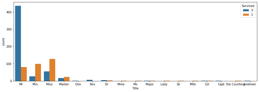

Mr : 많이 사망했다.
Mrs, Miss, Master 상대적으로 생존이 더 많음

train['Title'].unique()

array(['Mr', 'Mrs', 'Miss', 'Master', 'Don', 'Rev', 'Dr', 'Mme', 'Ms',
       'Major', 'Lady', 'Sir', 'Mlle', 'Col', 'Capt', 'the Countess',
       'Jonkheer'], dtype=object)

title = ['Mr', 'Mrs', 'Miss', 'Master', 'Rev','Don', 'Dr', 'Mme', 'Ms',
'Major', 'Lady', 'Sir', 'Mlle', 'Col', 'Capt', 'the Countess',
'Jonkheer']
# 데이터가 있는 ['Mr', 'Mrs', 'Miss', 'Master','Rev']만 사용하고 나머지는 Other로

len(title)

c_title = ['Mr', 'Mrs', 'Miss', 'Master','Rev'] + ['Other']*12
c_title

['Mr',
 'Mrs',
 'Miss',
 'Master',
 'Rev',
 'Other',
 'Other',
 'Other',
 'Other',
 'Other',
 'Other',
 'Other',
 'Other',
 'Other',
 'Other',
 'Other',
 'Other']

title_dict=dict(zip(title, c_title)) # zip함수를 이용해 title이 키값: c_title이 벨류값으로 -> 딕셔너리 형태로 만들어짐

title_dict

{'Mr': 'Mr',
 'Mrs': 'Mrs',
 'Miss': 'Miss',
 'Master': 'Master',
 'Rev': 'Rev',
 'Don': 'Other',
 'Dr': 'Other',
 'Mme': 'Other',
 'Ms': 'Other',
 'Major': 'Other',
 'Lady': 'Other',
 'Sir': 'Other',
 'Mlle': 'Other',
 'Col': 'Other',
 'Capt': 'Other',
 'the Countess': 'Other',
 'Jonkheer': 'Other'}

train['Title'] = train['Title'].map(title_dict)

train['Title'].value_counts()

Mr        517
Miss      182
Mrs       125
Master     40
Other      21
Rev         6
Name: Title, dtype: int64

title_dict['Dona'] = 'Other' # test에 있는 Dona를 추가
title_dict

test['Title'].unique()

array(['Mr', 'Mrs', 'Miss', 'Master', 'Ms', 'Col', 'Rev', 'Dr', 'Dona'],
      dtype=object)

test['Title'] = test['Title'].map(title_dict)

test['Title'].value_counts()

Mr        240
Miss       78
Mrs        72
Master     21
Other       5
Rev         2
Name: Title, dtype: int64

티켓

삭제

train.drop('Ticket', axis=1, inplace=True)
test.drop('Ticket', axis=1, inplace=True)

train.drop('Name', axis=1, inplace=True)
test.drop('Name', axis=1, inplace=True)

범주형 컬럼을 인코딩

y_train = train['Survived']
X_train = train.drop('Survived', axis = 1) #Survived 컬럼을 제외하고 넣는다
X_test = test

feature = ['Sex', 'Embarked', 'Deck', 'Title']

for i in feature:
    dummy = pd.get_dummies(train[i], prefix = i)
    X_train = pd.concat([X_train, dummy], axis=1)
    X_train.drop(i, axis=1, inplace = True)

for i in feature:
    dummy = pd.get_dummies(test[i], prefix = i)
    X_test = pd.concat([X_test, dummy], axis=1)
    X_test.drop(i, axis=1, inplace = True)

X_train.shape

(891, 26)

X_test.shape

(418, 25)

set(X_train.columns) - set(X_test.columns)

{'Deck_T'}

Deck_T가 X_test에 없는데, X_test['Deck_T'] = 0로 값이 없게 해준다

=> 원핫인코딩을 했기때문에 0은 없는값 1이 있는값

X_test['Deck_T'] = 0

set(X_train.columns) - set(X_test.columns)

set()

모델 선택 및 학습

from sklearn.neighbors import KNeighborsClassifier
from sklearn.tree import DecisionTreeClassifier

from sklearn.model_selection import cross_val_score # 교차검증

k_model = KNeighborsClassifier(n_neighbors=3)

result = cross_val_score(k_model, X_train, y_train, cv = 5)  # cv = 나눌횟수
result.mean()

0.7284162952733664

knn Scaler 적용 ( 더 높은 성능을 위해 knn시에 Scaler활용)

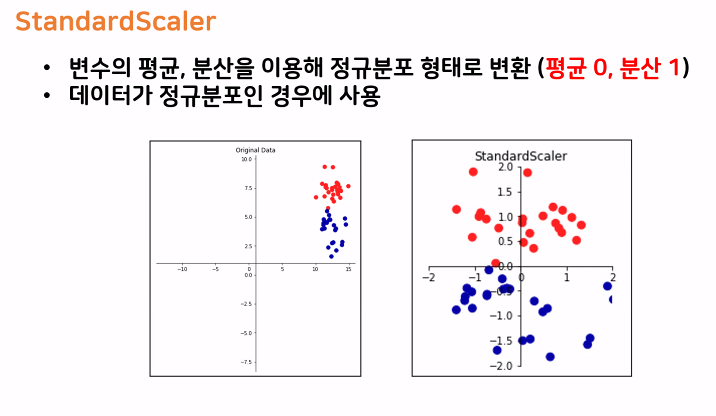
from sklearn.preprocessing import StandardScaler

scaler = StandardScaler()
scaler.fit(X_train)

StandardScaler()

t_X_train = scaler.transform(X_train)

t_X_test = scaler.transform(X_test) # train데이터로 fit하고 test도 바꿔준다

t_X_train

array([[ 0.82737724, -0.55136635,  0.43279337, ..., -0.4039621 ,
        -0.15536387, -0.0823387 ],
       ...,
       [ 0.82737724, -0.57020066,  0.43279337, ..., -0.4039621 ,
        -0.15536387, -0.0823387 ],
       [-1.56610693, -0.25001739, -0.4745452 , ..., -0.4039621 ,
        -0.15536387, -0.0823387 ],
       [ 0.82737724,  0.20200606, -0.4745452 , ..., -0.4039621 ,
        -0.15536387, -0.0823387 ]])

k_model = KNeighborsClassifier(n_neighbors=3)

result = cross_val_score(k_model, t_X_train, y_train, cv = 5) # cv = 나눌횟수
result.mean()

0.7946017199171427

tree 모델

max_depth =5

t_model = DecisionTreeClassifier(max_depth=5)

result = cross_val_score(t_model, X_train, y_train, cv = 5) # cv = 나눌횟수
result.mean()

0.8080911430544223

평가

케글사이트에 올려보자

sub = pd.read_csv('./data/titanic/gender_submission.csv')
sub

PassengerId	Survived
0	892	0
1	893	1
2	894	0
3	895	0
4	896	1
...	...	...
413	1305	0
414	1306	1
415	1307	0
416	1308	0
417	1309	0
418 rows × 2 columns

t_model.fit(X_train,y_train)
pre = t_model.predict(X_test)

sub['Survived'] = pre # Tree모델을 이용한 예측값을 Survived에 넣어준다

sub.to_csv('submission_01.csv', index = False)

트리모델 사용하여 영향을 많이끼친 특성 찾기

fi = t_model.feature_importances_

df = pd.DataFrame(fi, index = X_train.columns)
df.sort_values(by=0, ascending=False)

	0
Title_Mr	0.570337
Family	0.145146
Fare	0.121515
Pclass	0.052686
Age	0.043930
Title_Rev	0.029679
Title_Other	0.011395
....................
Deck_B	0.000000
Deck_A	0.000000
Embarked_Q	0.000000
Embarked_C	0.000000
Deck_F	0.000000

'빅데이터 서비스 교육 > 머신러닝' 카테고리의 다른 글

Linear Model 실습 (0)	2022.07.01
Linear Model (0)	2022.06.29
Cross validation (0)	2022.06.24
머신러닝 Decision Tree (0)	2022.06.24
Decision Tree (0)	2022.06.23

현재글예제 타이타닉 생존자 예측분석

오라클 19c, 오라클 클라우드, 활성화 함수, OCI, oracle adg, rman catalog, Deep Learning, 머신러닝, AZURE, 오라클 RAC, 리눅스, adg, RNN, 오라클 adg, 딥러닝, 전이학습, JavaScript, rman, Character set, 오라클,

Today :
Yesterday :

데이터들