보스턴 주택 값 예측 실습
import numpy as np
import pandas as pd
import matplotlib.pyplot as plt
from sklearn.datasets import load_boston # 보스턴 주택값 데이터
boston = load_boston()
boston_df = pd.DataFrame(boston.data, columns = boston.feature_names)
boston_df.head()
CRIM	ZN	INDUS	CHAS	NOX	RM	AGE	DIS	RAD	TAX	PTRATIO	B	LSTAT
0	0.00632	18.0	2.31	0.0	0.538	6.575	65.2	4.0900	1.0	296.0	15.3	396.90	4.98
1	0.02731	0.0	7.07	0.0	0.469	6.421	78.9	4.9671	2.0	242.0	17.8	396.90	9.14
2	0.02729	0.0	7.07	0.0	0.469	7.185	61.1	4.9671	2.0	242.0	17.8	392.83	4.03
3	0.03237	0.0	2.18	0.0	0.458	6.998	45.8	6.0622	3.0	222.0	18.7	394.63	2.94
4	0.06905	0.0	2.18	0.0	0.458	7.147	54.2	6.0622	3.0	222.0	18.7	396.90	5.33
train, test 분리
from sklearn.model_selection import train_test_split
X_train, X_test, y_train, y_test = train_test_split(boston_df, boston.target,
test_size =0.3,
random_state=1)
모델적용
from sklearn.linear_model import LinearRegression
from sklearn.model_selection import cross_val_score
l_model = LinearRegression()
l_model.fit(X_train, y_train)
LinearRegression()l_model.score(X_test,y_test)
0.7836295385076281print(l_model.coef_)
print(l_model.intercept_)
[-9.85424717e-02  6.07841138e-02  5.91715401e-02  2.43955988e+00       # 가중치의 개수는
 -2.14699650e+01  2.79581385e+00  3.57459778e-03 -1.51627218e+00       # 특성의 수와 같다
  3.07541745e-01 -1.12800166e-02 -1.00546640e+00  6.45018446e-03
 -5.68834539e-01]
46.396493871823864
result=cross_val_score(l_model, X_train,y_train, cv=5)
result.mean()
0.6643081077199126특성확장
e_X_train = X_train.copy()
for i in X_train.columns:
for j in X_train.columns:
e_X_train[i+'x'+j] = X_train[i] * X_train[j]
e_X_train.head()
CRIM	ZN	INDUS	CHAS	NOX	RM	AGE	DIS	RAD	TAX	...	LSTATxCHAS	LSTATxNOX	LSTATxRM	LSTATxAGE	LSTATxDIS	LSTATxRAD	LSTATxTAX	LSTATxPTRATIO	LSTATxB	LSTATxLSTAT
13	0.62976	0.0	8.14	0.0	0.538	5.949	61.8	4.7075	4.0	307.0	...	0.0	4.44388	49.13874	510.468	38.883950	33.04	2535.82	173.460	3278.3940	68.2276
61	0.17171	25.0	5.13	0.0	0.453	5.966	93.4	6.8185	8.0	284.0	...	0.0	6.54132	86.14904	1348.696	98.459140	115.52	4100.96	284.468	5459.4752	208.5136
377	9.82349	0.0	18.10	0.0	0.671	6.794	98.8	1.3580	24.0	666.0	...	0.0	14.25204	144.30456	2098.512	28.843920	509.76	14145.84	429.048	8430.1560	451.1376
39	0.02763	75.0	2.95	0.0	0.428	6.595	21.8	5.4011	3.0	252.0	...	0.0	1.84896	28.49040	94.176	23.332752	12.96	1088.64	79.056	1709.1216	18.6624
365	4.55587	0.0	18.10	0.0	0.718	3.561	87.9	1.6132	24.0	666.0	...	0.0	5.11216	25.35432	625.848	11.485984	170.88	4741.92	143.824	2525.4640	50.6944
5 rows × 182 columns
e_X_train.shape
(354, 182)l_model = LinearRegression()
l_model.fit(e_X_train, y_train)
LinearRegression()e_X_test = X_test.copy()
for i in X_test.columns:
for j in X_test.columns:
e_X_test[i+'x'+j] = X_test[i] * X_test[j]
l_model.score(e_X_test, y_test)
0.8043803930997194
Ridge (L2규제)
from sklearn.linear_model import Ridge
r_model = Ridge() # alpha= 로 규제의 강도 설정
r_model.fit(e_X_train, y_train)
r_model.score(e_X_test,y_test)
0.8239994029608095Ridge vs Lasso
from sklearn.linear_model import Lasso
alpha_list =[0.001, 0.01, 0.1, 10 , 100, 1000]
r_coef = []
l_coef = []
for i in alpha_list:
r_model = Ridge(alpha =i)
l_model = Lasso(alpha =i)
r_model.fit(e_X_train,y_train)
l_model.fit(e_X_train,y_train)
r_coef.append(r_model.coef_)
l_coef.append(l_model.coef_)
len(r_coef)
6
len(l_coef)
6
r_df = pd.DataFrame(np.array(r_coef).T, columns=alpha_list) #.T -> arrayList의 축을 바꿀때 사용
r_df
0.001	0.010	0.100	10.000	100.000	1000.000
0	-2.967946	-3.084029	-2.661836	-0.075861	-0.004695	0.000504
1	0.440672	0.414180	0.314357	-0.194214	-0.158361	-0.035165
2	-4.971540	-4.576505	-3.893822	-0.230469	0.007065	0.004058
3	37.790726	27.202270	7.193797	0.101728	0.005391	0.000041
4	42.723740	6.367370	0.419346	0.029559	0.005779	0.000777
...	...	...	...	...	...	...
177	-0.009413	-0.009255	-0.010853	-0.018205	-0.018827	-0.015527
178	-0.000908	-0.000899	-0.000819	0.000001	0.000127	-0.000010
179	0.019950	0.020062	0.021877	0.016719	0.012587	0.005452
180	-0.000297	-0.000308	-0.000322	-0.000315	-0.000292	-0.000085
181	0.015527	0.015380	0.015380	0.020819	0.025236	0.031515
182 rows × 6 columns
def plot(coef, alpha):
plt.figure(figsize = (20,5))
plt.bar(e_X_train.columns, coef)
plt.title('alpha ={}'.format(alpha))
plt.ylim([-13,5])
plt.show()
cnt = 0
for i in alpha_list:
plot(r_coef[cnt], i)
cnt+=1

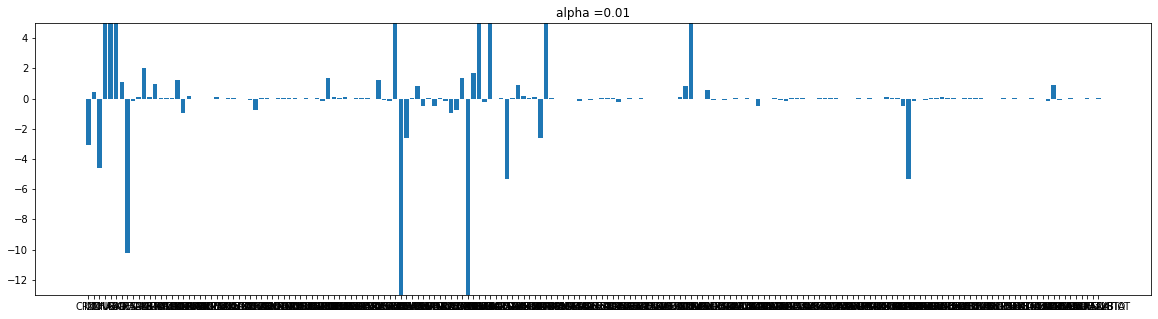
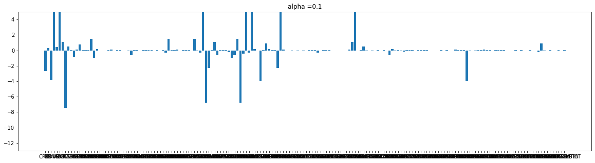
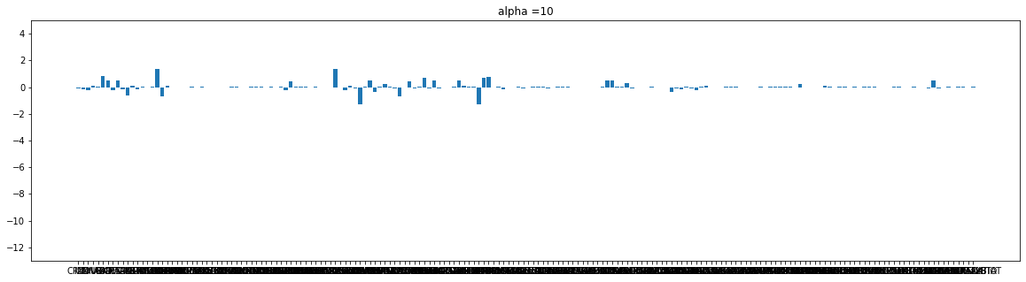
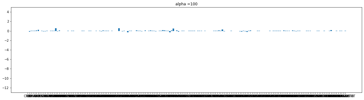
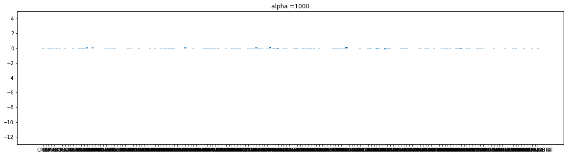
Ridge는 규제가 강해질수록 가중치가 작아진다.
cnt = 0
for i in alpha_list:
plot(l_coef[cnt], i)
cnt+=1
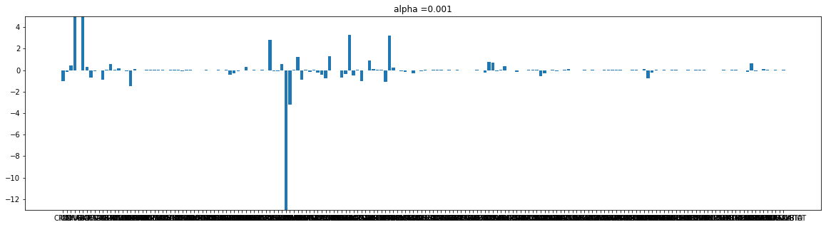
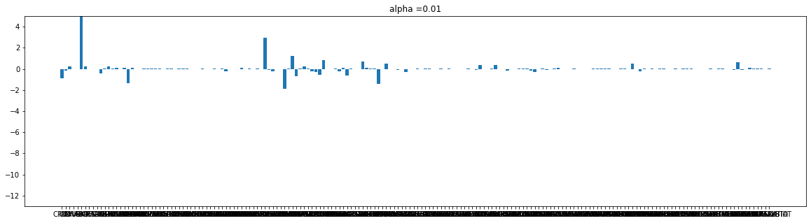
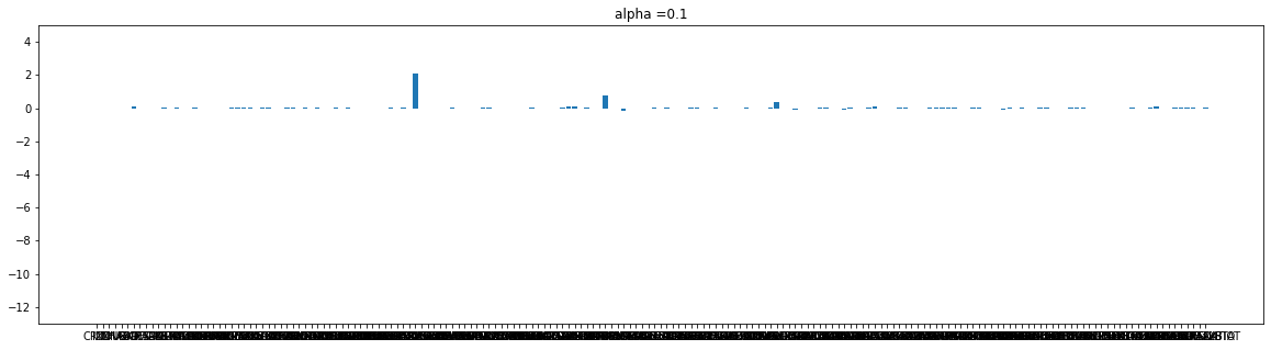
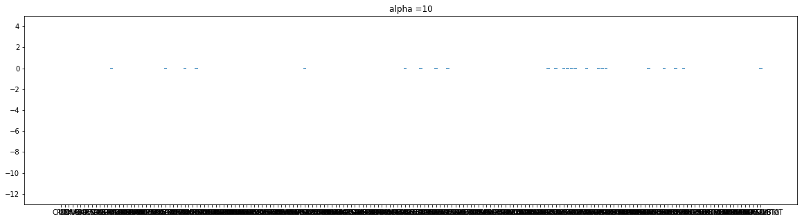
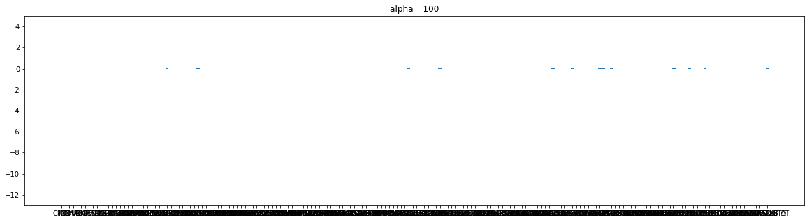
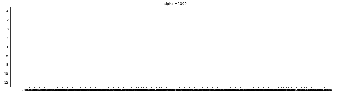
Lasso는 규제가 강해 질수록 가중치가 사라진다
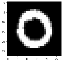
손글씨 분류 실습
목표
- 손 글씨 숫자(0~9)를 분류하는 모델을 만들어 보자.
- 이미지 데이터의 형태를 이해
import numpy as np
import pandas as pd
import matplotlib.pyplot as plt
data = pd.read_csv('./data/digit_train.csv')
data.head()
label	pixel0	pixel1	pixel2	pixel3	pixel4	pixel5	pixel6	pixel7	pixel8	...	pixel774	pixel775	pixel776	pixel777	pixel778	pixel779	pixel780	pixel781	pixel782	pixel783
0	1	0	0	0	0	0	0	0	0	0	...	0	0	0	0	0	0	0	0	0	0
1	0	0	0	0	0	0	0	0	0	0	...	0	0	0	0	0	0	0	0	0	0
2	1	0	0	0	0	0	0	0	0	0	...	0	0	0	0	0	0	0	0	0	0
3	4	0	0	0	0	0	0	0	0	0	...	0	0	0	0	0	0	0	0	0	0
4	0	0	0	0	0	0	0	0	0	0	...	0	0	0	0	0	0	0	0	0	0
5 rows × 785 columns
data.shape
(42000, 785)img0 = data.iloc[0,1:]
print(img0.max())
print(img0.min())
255
0
img0.values.reshape(28,28) # imshow 안에는 이미지를 넣어야 하므로
# 1차원인 img0을 2차원형태(28X28)로 reshape한다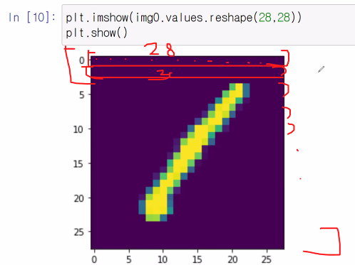
28개의 데이터 28줄
img1 = data.iloc[1,1:]
plt.imshow(img1.values.reshape(28,28), cmap='gray')
5000장 추출
X = data.iloc[:5000,1:]
y = data.iloc[:5000,0]
print(X.shape)
print(y.shape)
(5000, 784)
(5000,)from sklearn.model_selection import train_test_split
X_train, X_test, y_train,y_test = train_test_split(X,y,test_size=0.3, random_state=1)
모델설계
- KNN
- Decision tree
- Logisitc regression
- SVM
from sklearn.neighbors import KNeighborsClassifier
from sklearn.tree import DecisionTreeClassifier
from sklearn.linear_model import LogisticRegression
from sklearn.svm import LinearSVC

knn = KNeighborsClassifier()
tree = DecisionTreeClassifier()
logi = LogisticRegression()
svm = LinearSVC()

knn.fit(X_train,y_train)
tree.fit(X_train,y_train)
logi.fit(X_train,y_train)
svm.fit(X_train,y_train)

print('knn : ',knn.score(X_test,y_test))
print('tree : ',tree.score(X_test,y_test))
print('logi : ',logi.score(X_test,y_test))
print('svm : ',svm.score(X_test,y_test))
knn : 0.914
tree : 0.7426666666666667
logi : 0.872
svm : 0.812스케일링
from sklearn.preprocessing import MinMaxScaler
Mms = MinMaxScaler()
Mms.fit(X_train)

X_train_s = Mms.transform(X_train)
X_test_s = Mms.transform(X_test)

knn.fit(X_train_s,y_train)
tree.fit(X_train_s,y_train)
logi.fit(X_train_s,y_train)
svm.fit(X_train_s,y_train)

print('knn : ',knn.score(X_test_s,y_test))
print('tree : ',tree.score(X_test_s,y_test))
print('logi : ',logi.score(X_test_s,y_test))
print('svm : ',svm.score(X_test_s,y_test))
knn : 0.914
tree : 0.746
logi : 0.882
svm : 0.8433333333333334예측
img5 = X_test_s[5]
knn.predict([img5]) # img5는 1차원 -> [img5]로 2차원으로 만들어준다(fit했을때와 동일한형태로)
array([9], dtype=int64)y_test[5] #답이 예측과 다른값
0array([[0. , 0. , 0. , 0. , 0. , 0. , 1. , 0. , 0. , 0. ],
[0. , 1. , 0. , 0. , 0. , 0. , 0. , 0. , 0. , 0. ],
[0. , 0. , 0. , 0. , 0.2, 0. , 0. , 0.8, 0. , 0. ],
[0. , 0. , 0. , 0. , 0. , 1. , 0. , 0. , 0. , 0. ],
[0. , 0. , 0. , 0. , 0. , 0. , 0. , 0. , 1. , 0. ],
[0. , 0. , 1. , 0. , 0. , 0. , 0. , 0. , 0. , 0. ],
[0. , 1. , 0. , 0. , 0. , 0. , 0. , 0. , 0. , 0. ],
[0. , 0. , 1. , 0. , 0. , 0. , 0. , 0. , 0. , 0. ],
[0. , 0.4, 0.6, 0. , 0. , 0. , 0. , 0. , 0. , 0. ],
[0. , 0. , 1. , 0. , 0. , 0. , 0. , 0. , 0. , 0. ],
[1. , 0. , 0. , 0. , 0. , 0. , 0. , 0. , 0. , 0. ],
[1. , 0. , 0. , 0. , 0. , 0. , 0. , 0. , 0. , 0. ],
[0. , 0. , 0. , 0. , 0. , 0. , 0. , 1. , 0. , 0. ],
[0. , 0. , 0. , 0. , 0. , 1. , 0. , 0. , 0. , 0. ],
[0. , 0. , 0. , 0.2, 0. , 0.2, 0. , 0. , 0.6, 0. ],
[0. , 0. , 0. , 0. , 0. , 0. , 1. , 0. , 0. , 0. ],
[1. , 0. , 0. , 0. , 0. , 0. , 0. , 0. , 0. , 0. ],
[1. , 0. , 0. , 0. , 0. , 0. , 0. , 0. , 0. , 0. ],
[0. , 0. , 0. , 0. , 1. , 0. , 0. , 0. , 0. , 0. ],
[0. , 0. , 0. , 0. , 0. , 0. , 0. , 0. , 1. , 0. ]])순서대로 1 2 3 4 5 6 7 8 9 일 확률을 예측한다 -> 그래서 가장 높은 확률인 숫자를 예측값으로 반환한다.
분류평가지표
from sklearn.metrics import classification_report
pre = knn.predict(X_test_s)
print(classification_report(pre,y_test))
print(classification_report(pre,y_test))
print(classification_report(pre,y_test))
              precision    recall  f1-score   support

           0       0.98      0.93      0.95       165
           1       0.99      0.83      0.90       172
           2       0.85      0.97      0.91       155
           3       0.91      0.91      0.91       149
           4       0.92      0.95      0.93       136
           5       0.93      0.90      0.91       146
           6       0.97      0.94      0.95       156
           7       0.90      0.92      0.91       151
           8       0.78      0.97      0.87       120
           9       0.91      0.86      0.89       150

    accuracy                           0.91      1500
   macro avg       0.92      0.92      0.91      1500
weighted avg       0.92      0.91      0.91      1500

# f1-score : 재현율, 정밀도 둘다 고려한 수치
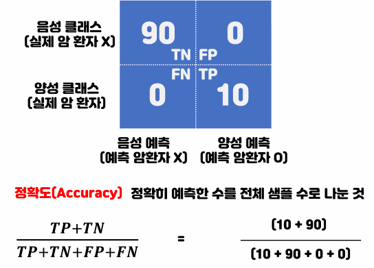
분류평가지표
오차행렬
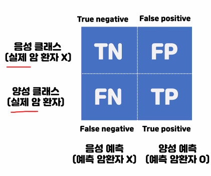
Y축 클래스 : 답
X축 예측 : 예측값
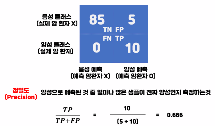
정밀도
재현율
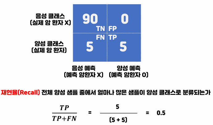

예측 결과가 잘못되었을때 큰 위험이 있을때(실제 상황에대한 리스크가 클때) -> 높은 재현율이 필요
모델이 예측 할때 비용이 많이 들때(모델에 대한 리스크[ex 비용이클때]가 클때) -> 높은 정밀도 필요
'빅데이터 서비스 교육 > 머신러닝' 카테고리의 다른 글
| 텍스트 마이닝 (0) | 2022.07.06 |
|---|---|
| 앙상블 모델 (0) | 2022.07.05 |
| Linear Model (0) | 2022.06.29 |
| 예제 타이타닉 생존자 예측분석 (0) | 2022.06.24 |
| Cross validation (0) | 2022.06.24 |