반응형
목표
- 학생 수학 성적을 예측하는 회귀 모델을 만들어 보자!
- keras를 이용해 신경망을 구성하는 방법을 익혀보자~
import numpy as np
import pandas as pd
import matplotlib.pyplot as plt
# delimiter : 데이터 파일에서 구분자를 설정해주는 명령
data = pd.read_csv('/content/drive/MyDrive/Colab Notebooks/빅데이터 13차(딥러닝)/Data/student-mat.csv', delimiter=";")
data
	school	sex	age	address	famsize	Pstatus	Medu	Fedu	Mjob	Fjob	...	famrel	freetime	goout	Dalc	Walc	health	absences	G1	G2	G3
0	GP	F	18	U	GT3	A	4	4	at_home	teacher	...	4	3	4	1	1	3	6	5	6	6
1	GP	F	17	U	GT3	T	1	1	at_home	other	...	5	3	3	1	1	3	4	5	5	6
2	GP	F	15	U	LE3	T	1	1	at_home	other	...	4	3	2	2	3	3	10	7	8	10
3	GP	F	15	U	GT3	T	4	2	health	services	...	3	2	2	1	1	5	2	15	14	15
4	GP	F	16	U	GT3	T	3	3	other	other	...	4	3	2	1	2	5	4	6	10	10
...	...	...	...	...	...	...	...	...	...	...	...	...	...	...	...	...	...	...	...	...	...
390	MS	M	20	U	LE3	A	2	2	services	services	...	5	5	4	4	5	4	11	9	9	9
391	MS	M	17	U	LE3	T	3	1	services	services	...	2	4	5	3	4	2	3	14	16	16
392	MS	M	21	R	GT3	T	1	1	other	other	...	5	5	3	3	3	3	3	10	8	7
393	MS	M	18	R	LE3	T	3	2	services	other	...	4	4	1	3	4	5	0	11	12	10
394	MS	M	19	U	LE3	T	1	1	other	at_home	...	3	2	3	3	3	5	5	8	9	9
395 rows × 33 columns
# 데이터 프레임에서 모든 컬럼 표시 (None: 모든 컬럼을 전부 표시함)
pd.set_option("display.max_columns", None)
school	sex	age	address	famsize	Pstatus	Medu	Fedu	Mjob	Fjob	reason	guardian	traveltime	studytime	failures	schoolsup	famsup	paid	activities	nursery	higher	internet	romantic	famrel	freetime	goout	Dalc	Walc	health	absences	G1	G2	G3
0	GP	F	18	U	GT3	A	4	4	at_home	teacher	course	mother	2	2	0	yes	no	no	no	yes	yes	no	no	4	3	4	1	1	3	6	5	6	6
1	GP	F	17	U	GT3	T	1	1	at_home	other	course	father	1	2	0	no	yes	no	no	no	yes	yes	no	5	3	3	1	1	3	4	5	5	6
2	GP	F	15	U	LE3	T	1	1	at_home	other	other	mother	1	2	3	yes	no	yes	no	yes	yes	yes	no	4	3	2	2	3	3	10	7	8	10
3	GP	F	15	U	GT3	T	4	2	health	services	home	mother	1	3	0	no	yes	yes	yes	yes	yes	yes	yes	3	2	2	1	1	5	2	15	14	15
4	GP	F	16	U	GT3	T	3	3	other	other	home	father	1	2	0	no	yes	yes	no	yes	yes	no	no	4	3	2	1	2	5	4	6	10	10
...	...	...	...	...	...	...	...	...	...	...	...	...	...	...	...	...	...	...	...	...	...	...	...	...	...	...	...	...	...	...	...	...	...
390	MS	M	20	U	LE3	A	2	2	services	services	course	other	1	2	2	no	yes	yes	no	yes	yes	no	no	5	5	4	4	5	4	11	9	9	9
391	MS	M	17	U	LE3	T	3	1	services	services	course	mother	2	1	0	no	no	no	no	no	yes	yes	no	2	4	5	3	4	2	3	14	16	16
392	MS	M	21	R	GT3	T	1	1	other	other	course	other	1	1	3	no	no	no	no	no	yes	no	no	5	5	3	3	3	3	3	10	8	7
393	MS	M	18	R	LE3	T	3	2	services	other	course	mother	3	1	0	no	no	no	no	no	yes	yes	no	4	4	1	3	4	5	0	11	12	10
394	MS	M	19	U	LE3	T	1	1	other	at_home	course	father	1	1	0	no	no	no	no	yes	yes	yes	no	3	2	3	3	3	5	5	8	9	9
395 rows × 33 columns
# 문제, 정답 분리
X = data['studytime'] # 문제
y = data['G3']
X.shape, y.shape
((395,), (395,))
# 학습, 평가 데이터 분리
from sklearn.model_selection import train_test_split
X_train, X_test, y_train, y_test = train_test_split(X,y,
test_size=0.3,
random_state=5
)
print(X_train.shape)
print(X_test.shape)
print(y_train.shape)
print(y_test.shape)
(276,) (119,) (276,) (119,)
신경망 모델 만들기!
-
- 신경망 구조 설계
- 신경망 학습 및 평가방법 설정
- 학습 / 시각화
- 모델 평가
# Sequential : 신경망의 뼈대를 구축하기 위한 모듈
from tensorflow.keras import Sequential
# InputLayer : 신경망의 입력층을 생성(데이터가 들어오는 입구 부분)
# Dense : 신경망에서 뉴런들의 묶음을 생성(층을 쌓아주는 역할)
from tensorflow.keras.layers import InputLayer, Dense
# 1. 신경망 구조 설계
# 신경망 뼈대 설정
model = Sequential()
# 입력층 설정
# input_shape : 입력 데이터의 특성 형태를 설정(특성이 1개면 1) input_shape=(1,) 뒤쪽은 차원으로 1차원이 기본값
model.add(InputLayer(input_shape=(1,)))
# 출력층 설정
# Dense(1) 안의 숫자는 하나의 층에 생성해줄 뉴런의 수
model.add(Dense(1))
# 설계된 신경망의 정보를 요약해서 출력
model.summary()
Model: "sequential"
_________________________________________________________________
 Layer (type)                Output Shape              Param #
=================================================================
 dense (Dense)               (None, 1)                 2

=================================================================
Total params: 2
Trainable params: 2
Non-trainable params: 0
_________________________________________________________________
# 2. 신경망 학습 및 평가방법 설정
model.compile(loss='mse', # 손실함수(=비용함수): MSE(평균제곱오차), 회귀문제이기 때문에 MSE를 사용
optimizer='SGD' # 최적화함수 : 경사하강법의 방법을 설정(SGD: 확률적 경사하강법), 딥러닝에서는 최소 SGD이상 사용
)
# 3. 학습
h = model.fit(X_train,y_train,
epochs=100 # epochs : 학습 횟수 설정
)
Epoch 1/100
9/9 [==============================] - 1s 3ms/step - loss: 65.7110
Epoch 2/100
9/9 [==============================] - 0s 3ms/step - loss: 32.5506
Epoch 3/100
9/9 [==============================] - 0s 4ms/step - loss: 28.4692
Epoch 4/100
9/9 [==============================] - 0s 3ms/step - loss: 27.7098
Epoch 5/100
9/9 [==============================] - 0s 3ms/step - loss: 27.4299
Epoch 6/100
9/9 [==============================] - 0s 4ms/step - loss: 27.1007
.................................................................
Epoch 96/100
9/9 [==============================] - 0s 2ms/step - loss: 20.4975
Epoch 97/100
9/9 [==============================] - 0s 3ms/step - loss: 20.5453
Epoch 98/100
9/9 [==============================] - 0s 3ms/step - loss: 20.5530
Epoch 99/100
9/9 [==============================] - 0s 3ms/step - loss: 20.4992
Epoch 100/100
9/9 [==============================] - 0s 3ms/step - loss: 20.5292
# 3. 시각화
plt.figure(figsize=(15,5))
# 라인 차트 생성
plt.plot(h.history['loss'],
label='loss'
)
plt.legend()
plt.show()
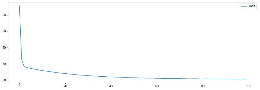
- 초반에는 빠르게 loss값(MSE)이 떨어지고 있음
- 경사하강법 초반에는 가중치(w), 절편(b)값이 임의의 값으로 설정 되어 있기 때문에 몇 번만 학습시켜도 빠르게 MSE가 줄어드는 것을 확인 할 수 있음
# 4. 모델 평가
model.evaluate(X_test,y_test)
4/4 [==============================] - 0s 4ms/step - loss: 21.9513
21.951276779174805
입력 특성이 2개인 신경망 모델을 만들어 보자
- 문제(입력특성 2개 : studytime, traveltime -X1
- 정답(G3) - y1
- 최종 출력층 뉴런의 개수는 1개
X1 = data[['studytime','traveltime']]  # 여러개의 특성을 넣을땐  ->  [[ 여러개 특성 ]]
y1 = data['G3']

X1_train, X1_test, y1_train, y1_test = train_test_split(X1,y1,
                                                        test_size = 0.3,
                                                        random_state = 5
                                                        )
model1 = Sequential()

model1.add(InputLayer(input_shape=(2,)))

model1.add(Dense(1))

# 학습 / 평가 방법 설정
model1.compile(loss='mse',
               optimizer='SGD')

# 학습
h1 = model1.fit(X1_train,y1_train,
           epochs=100)

plt.figure(figsize=(15,5))

plt.plot(h1.history['loss'],
         label='loss')

plt.legend()
plt.show()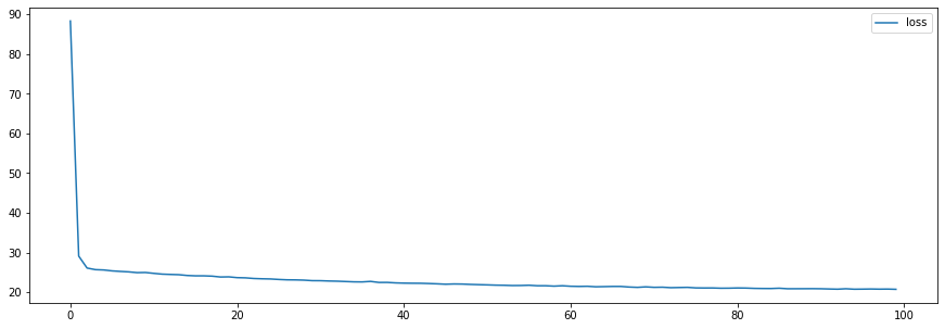
model1.evaluate(X1_test, y1_test)
4/4 [==============================] - 0s 3ms/step - loss: 22.4100
22.409971237182617
반응형
'빅데이터 서비스 교육 > 딥러닝' 카테고리의 다른 글
| 활성화함수 (0) | 2022.07.14 |
|---|---|
| 딥러닝 유방암 데이터 분류 예제 (0) | 2022.07.14 |
| 딥러닝 2진분류 실습 (폐암환자 예측) (0) | 2022.07.13 |
| 퍼셉트론, 다층 퍼셉트론 (0) | 2022.07.13 |
| 딥러닝 (0) | 2022.07.12 |