반응형
목표
- 재우, 감중 얼굴을 분류하는 이진 분류 신경망 모델을 만들어보자
import numpy as np
import pandas as pd
import matplotlib.pyplot as plt
from PIL import Image # PIL : 이미지를 불러오는 라이브러리
# convert -> L : 흑백, RGB : 컬러
img = Image.open("/content/drive/MyDrive/Colab Notebooks/빅데이터 13차(딥러닝)/Data/Class 1-samples/0.jpg").convert('L')
img

# numpy 배열로 이미지 데이터를 변환(기계가 인식할 수 있또록 데이터를 수치화 시켜줌)
# 이미지의 크기에 맞게 가로, 세로 픽셀수로 수치화가 됨
img_array = np.array(img)
img_array
array([[123, 125, 129, ..., 253, 254, 254],
       [127, 127, 130, ..., 254, 254, 254],
       [129, 129, 130, ..., 254, 253, 254],
       ...,
       [123, 122, 122, ..., 155, 154, 152],
       [123, 122, 121, ..., 155, 154, 152],
       [122, 120, 119, ..., 154, 153, 150]], dtype=uint8)
img_array.shape
(224, 224)# 반복문 실행시 어느정도 실행되고 있는지 %로 알려주는 라이브러리
from tqdm import tqdm
# 학습 데이터셋 구성하기
class1_list = [] #재우 데이터가 들어갈 자리
class2_list = [] #감중 데이터가 들어갈 자리
for i in tqdm(range(0,200,1)):
# 1. 재우 데이터 작업
# 경로와 이름에 맞게 이미지를 가져와서 흑백으로 변환 후 img1 변수에 담아주기
img1 = Image.open(f"/content/drive/MyDrive/Colab Notebooks/빅데이터 13차(딥러닝)/Data/Class 1-samples/{str(i)}.jpg").convert('L')
img_array1 = np.array(img1)
# numpy배열 데이터를 빈 리스트에 하나씩 추가해주기
class1_list.append(img_array1)
# 2. 감중 데이터 작업
img2 = Image.open(f"/content/drive/MyDrive/Colab Notebooks/빅데이터 13차(딥러닝)/Data/Class 2-samples/{str(i)}.jpg").convert('L')
img_array2 = np.array(img2)
# numpy배열 데이터를 빈 리스트에 하나씩 추가해주기
class2_list.append(img_array2)
100%|██████████| 200/200 [00:34<00:00, 5.75it/s]
class1_list
        ...............................................
        [126, 124, 125, ..., 153, 154, 154],
        [125, 123, 124, ..., 153, 153, 153],
        [124, 123, 123, ..., 153, 153, 152]], dtype=uint8),
 array([[127, 130, 129, ..., 254, 253, 253],
        [127, 130, 129, ..., 254, 253, 253],
        [128, 130, 129, ..., 253, 254, 253],
        ...,
        [126, 126, 125, ..., 153, 154, 153],
        [125, 125, 124, ..., 153, 154, 152],
        [123, 124, 124, ..., 153, 154, 151]], dtype=uint8)]
# 리스트 자체도 numpy배열로 변환
# 사진 하나하나도 numpy배열로, 이를 담은 리스트도 numpy배열로 변환시켜줘야 한다 (신경망에 들어갈 수 있는 형태로 변경시켜주기 위함)
class1_numpy = np.array(class1_list)
class2_numpy = np.array(class2_list)
class1_numpy
array([[[123, 125, 129, ..., 253, 254, 254],
        [127, 127, 130, ..., 254, 254, 254],
        [129, 129, 130, ..., 254, 253, 254],
        ...,
        [123, 122, 122, ..., 155, 154, 152],
        [123, 122, 121, ..., 155, 154, 152],
        [122, 120, 119, ..., 154, 153, 150]],

       [[127, 128, 130, ..., 254, 254, 254],
        [127, 127, 130, ..., 254, 254, 253],
        [129, 128, 130, ..., 254, 254, 253],

        ....................................
# concatenate : 두 배열을 순서대로 붙여주는 명령
data = np.concatenate((class1_numpy,class2_numpy))
class1_numpy.shape, data.shape
((200, 224, 224), (400, 224, 224))# 정답 데이터 만들기(문제와 정답의 순서를 일정하게 맞춰줄 것)
# 0을 재우 데이터의 정답으로, 1을 감중 데이터의 정답으로 해보자
target = np.array([0]*200 + [1]*200)
target
array([0, 0, 0, 0, 0, 0, 0, 0, 0, 0, 0, 0, 0, 0, 0, 0, 0, 0, 0, 0, 0, 0,
       0, 0, 0, 0, 0, 0, 0, 0, 0, 0, 0, 0, 0, 0, 0, 0, 0, 0, 0, 0, 0, 0,
       0, 0, 0, 0, 0, 0, 0, 0, 0, 0, 0, 0, 0, 0, 0, 0, 0, 0, 0, 0, 0, 0,
       0, 0, 0, 0, 0, 0, 0, 0, 0, 0, 0, 0, 0, 0, 0, 0, 0, 0, 0, 0, 0, 0,
       0, 0, 0, 0, 0, 0, 0, 0, 0, 0, 0, 0, 0, 0, 0, 0, 0, 0, 0, 0, 0, 0,
       0, 0, 0, 0, 0, 0, 0, 0, 0, 0, 0, 0, 0, 0, 0, 0, 0, 0, 0, 0, 0, 0,
       0, 0, 0, 0, 0, 0, 0, 0, 0, 0, 0, 0, 0, 0, 0, 0, 0, 0, 0, 0, 0, 0,
       0, 0, 0, 0, 0, 0, 0, 0, 0, 0, 0, 0, 0, 0, 0, 0, 0, 0, 0, 0, 0, 0,
       0, 0, 0, 0, 0, 0, 0, 0, 0, 0, 0, 0, 0, 0, 0, 0, 0, 0, 0, 0, 0, 0,
       0, 0, 1, 1, 1, 1, 1, 1, 1, 1, 1, 1, 1, 1, 1, 1, 1, 1, 1, 1, 1, 1,
       1, 1, 1, 1, 1, 1, 1, 1, 1, 1, 1, 1, 1, 1, 1, 1, 1, 1, 1, 1, 1, 1,
       1, 1, 1, 1, 1, 1, 1, 1, 1, 1, 1, 1, 1, 1, 1, 1, 1, 1, 1, 1, 1, 1,
       1, 1, 1, 1, 1, 1, 1, 1, 1, 1, 1, 1, 1, 1, 1, 1, 1, 1, 1, 1, 1, 1,
       1, 1, 1, 1, 1, 1, 1, 1, 1, 1, 1, 1, 1, 1, 1, 1, 1, 1, 1, 1, 1, 1,
       1, 1, 1, 1, 1, 1, 1, 1, 1, 1, 1, 1, 1, 1, 1, 1, 1, 1, 1, 1, 1, 1,
       1, 1, 1, 1, 1, 1, 1, 1, 1, 1, 1, 1, 1, 1, 1, 1, 1, 1, 1, 1, 1, 1,
       1, 1, 1, 1, 1, 1, 1, 1, 1, 1, 1, 1, 1, 1, 1, 1, 1, 1, 1, 1, 1, 1,
       1, 1, 1, 1, 1, 1, 1, 1, 1, 1, 1, 1, 1, 1, 1, 1, 1, 1, 1, 1, 1, 1,
       1, 1, 1, 1])
data.shape, target.shape
((400, 224, 224), (400,))from sklearn.model_selection import train_test_split
# train_test_split으로 데이터를 랜덤하게 섞었다
X_train, X_test, y_train, y_test = train_test_split(data, target,
test_size=0.2,
random_state=1
)
print(X_train.shape)
print(X_test.shape)
print(y_train.shape)
print(y_test.shape)
(320, 224, 224)
(80, 224, 224)
(320,)
(80,)
신경망 모델링
- 재우, 감중 이미지를 분류하는 신경망 모델 설계
from tensorflow.keras import Sequential
from tensorflow.keras.layers import Dense, Flatten

model = Sequential()

model.add(Flatten(input_shape=(224,224)))

model.add(Dense(500, activation="relu"))
model.add(Dense(300, activation="relu"))
model.add(Dense(100, activation="relu"))

model.add(Dense(1, activation="sigmoid"))

model.compile(loss="binary_crossentropy",
              optimizer="Adam",
              metrics=['acc'])

h = model.fit(X_train,y_train,
              validation_split=0.2,
              epochs=100,
              batch_size=128)

# validation_split : 자동으로 train 데이터에서 검증 데이터를 분리시켜주는 명령
# 주의점 : 분리시켜줄 때 뒤에서부터 20%를 잘라줌
#          일정한 값으로 정렬돼 있는 데이터에는 사용할 수 없음(데이터가 섞여있어야 한다)
Epoch 1/100
2/2 [==============================] - 1s 311ms/step - loss: 0.0000e+00 - acc: 1.0000 - val_loss: 0.0000e+00 - val_acc: 1.0000
Epoch 2/100
2/2 [==============================] - 0s 39ms/step - loss: 0.0000e+00 - acc: 1.0000 - val_loss: 0.0000e+00 - val_acc: 1.0000
Epoch 3/100
2/2 [==============================] - 0s 39ms/step - loss: 0.0000e+00 - acc: 1.0000 - val_loss: 0.0000e+00 - val_acc: 1.0000
Epoch 4/100
2/2 [==============================] - 0s 38ms/step - loss: 0.0000e+00 - acc: 1.0000 - val_loss: 0.0000e+00 - val_acc: 1.0000
Epoch 5/100
2/2 [==============================] - 0s 36ms/step - loss: 0.0000e+00 - acc: 1.0000 - val_loss: 0.0000e+00 - val_acc: 1.0000
...........................................................................................................................
Epoch 100/100
2/2 [==============================] - 0s 36ms/step - loss: 0.0000e+00 - acc: 1.0000 - val_loss: 0.0000e+00 - val_acc: 1.0000plt.figure(figsize=(15,5))
# train 데이터
plt.plot(h.history['acc'],
label='acc',
c = 'blue',
marker='.'
)
# val 데이터
plt.plot(h.history['val_acc'],
label='val_acc',
c = 'red',
marker='.'
)
plt.xlabel("epochs")
plt.ylabel("accuracy")
plt.legend()
plt.show()
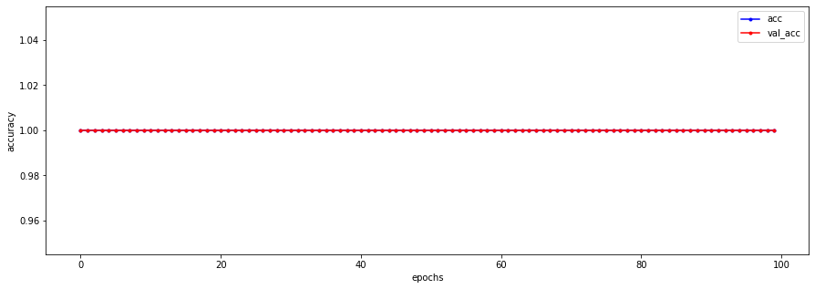
- 같은배경, 사람의 위치도 크게 변하지 않아서 학습하기 쉬운 데이터라 정확도 100%가 나왔다.
model.evaluate(X_test, y_test)
3/3 [==============================] - 0s 24ms/step - loss: 0.0000e+00 - acc: 1.0000
[0.0, 1.0]
반응형
'빅데이터 서비스 교육 > 딥러닝' 카테고리의 다른 글
| 활성화함수, 최적화함수 비교 및 최적화 모델 찾기 (0) | 2022.07.21 |
|---|---|
| 활성화함수, 최적화 함수 (0) | 2022.07.19 |
| 이미지 데이터 분류 (0) | 2022.07.18 |
| 딥러닝 iris 데이터 신경망으로 풀기 (다중 분류) (0) | 2022.07.14 |
| 활성화함수 (0) | 2022.07.14 |